
Independent engineering case study
Thermal-runaway exhaust plume.
A reconstructed aircraft center section and a prescribed hot-gas pulse show how exhaust interacts with the fuselage and ground, spreads, and disperses after venting stops.
By Mohammadreza Khani, PhD · Khani Solutions · Illustrative numerical simulation
The video is a presentation of solver results. Assumptions, numerical checks and interpretation are documented below.
More details — full technical case studyFewer details — close technical case study
The engineering challenge
Routing battery vent gas outside an aircraft is only part of the problem. Once a hot jet leaves the outlet, its momentum, buoyancy, the fuselage shape, and the nearby ground determine where it travels. A downward-facing vent can move the initial release away from the cabin yet create a hot region below the aircraft. The plume can spread along the ground, entrain surrounding air, and turn upward as it loses momentum.
I built this external-flow study to make those interactions visible for a stationary aircraft on the ground. The purpose is to establish a repeatable geometry-to-results workflow for examining a hypothetical thermal-runaway exhaust release. The model helps frame questions about outlet placement, clearance, local recirculation, and the persistence of hot gas after venting stops.
This is an independent Khani Solutions portfolio demonstration using an approximate Archer Midnight-inspired body reconstructed from public images. The outlet and release conditions are my assumptions. It is not an Archer or Wisk design analysis, employer project, certification result, or assessment of either company's battery safety.
What was modeled
The calculation resolves only the air outside a vertical, longitudinal aircraft center section. A prescribed hot-gas boundary represents exhaust that has already left the battery system. Cell failure, pack pressure, gas generation, propagation, and the internal vent duct are not solved. Consequently, the simulation predicts external flow and gas temperature for the specified release; it does not predict whether thermal runaway occurs or what a real pack would discharge.
Thermal-runaway exhaust can involve composition changes, combustible gases and particles. Here it is represented as a single nonreacting, air-like gas. The colored field is gas temperature, rather than a species concentration, flame, smoke-density field, or toxic-exposure measure.
Step 1 — Reconstruct and review the center section
I compared public side, front three-quarter, rear three-quarter, and elevated views of the black Midnight aircraft. An early side outline included features that lie outside the center plane. I replaced it with an estimated three-dimensional fuselage envelope built from 17 cross-sectional stations in FreeCAD, then intersected that envelope at the lateral coordinate y = 0. This produces a nose-to-tail center cut rather than using the entire projected side silhouette as a solid CFD obstruction.
The estimated fuselage is 7.2 m long. Image scaling uses an assumed 8.2 m projected whole-aircraft nose-to-tail-tip extent. Those dimensions, hidden contours, cross-sectional widths, and an assumed centered nose fairing are reconstruction inputs, not manufacturer measurements. The wing attachment is blended into the roof estimate. Off-center main landing-gear fairings, wing and rotor booms, and V-tail arms are excluded from the solved plane.
I overlaid the center cut on the reference image and reviewed the estimated envelope from multiple views before meshing. The approved 25 mm clearance beneath the assumed nose fairing was retained; the model does not establish actual tire contact. CAD validity, section planarity, and the exposed 100 mm vent edge were checked. The native FreeCAD and STEP geometry uses millimetres; the CFD geometry uses metres.
Step 2 — Define a hypothetical ground release
| Input | Value used |
|---|---|
| Aircraft and rotors | Stationary, on the ground; rotors stopped |
| Ambient | Still air at 25°C; hydrostatic pressure referenced to 101,325 Pa at ground level |
| Gravity | 9.81 m/s² downward |
| Outlet | 100 mm flush belly slot, centered at longitudinal x ≈ 4.9000 m and height ≈ 0.7004 m; x increases from nose toward tail |
| Exhaust temperature | 600°C (873.15 K) |
| Jet velocity | 40 m/s, directed 35° aft and downward; components (32.7661, −22.9431, 0) m/s in solver coordinates |
| Release timing | 0–10 s venting, then a closed no-slip adiabatic mouth and 5 s additional dispersion |
| Walls and ground | Stationary, no slip, adiabatic |
| External domain | Longitudinal x = −16.4 to 32.8 m; height = 0 to 24.6 m |
| 2D representation | One cell through a 0.1 m extrusion; front/back boundaries are empty |
The prescribed release is an illustrative pulse. Closing the mouth at 10 s is also an assumed scenario, not a model of a real vent valve. A 2D slot represents flow per unit span; it is not a 100 mm diameter nozzle. Normal mass flux depends on the local slot normal as well as jet direction, so this case is not a controlled mass-flow comparison with the earlier protruding-outlet concept.
Step 3 — Generate and check the external-fluid mesh
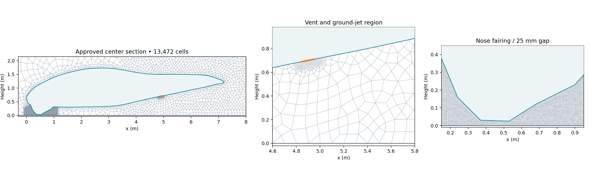
Gmsh 4.15.2 generated the external-air mesh around the approved section. The wall was simplified to remove very short construction segments while preserving the vent endpoints. Maximum boundary deviation from the CAD cut was approximately 0.952 mm. The mesh contains 13,472 finite-volume cells and eight faces across the outlet, with a single cell through the span.
Target sizes were 12.5 mm near the vent, 6 mm around the nose-fairing gap, approximately 80 mm near the body, 100 mm in the near-ground release zone, 230 mm in the wider plume region, and up to 1.5 m in the far field. The local targets focus resolution on the source, clearances, and initial ground interaction. No dedicated wall-normal boundary-layer stack was established; wall functions were used, and wall-resolution independence was not demonstrated.
OpenFOAM's checkMesh -allTopology -allGeometry returned Mesh OK. Maximum non-orthogonality was 44.54° and maximum skewness was 1.57. These checks support a usable numerical mesh; they do not establish grid-independent plume temperatures.
Step 4 — Set up the flow and thermal solver
I used OpenCFD OpenFOAM v2506 buoyantPimpleFoam for transient compressible, buoyant, nonreacting flow with sensible-enthalpy transport. Density follows the perfect-gas equation of state, allowing the hot exhaust to be less dense than ambient air. The gas molecular weight is 28.965 kg/kmol, with constant specific heat Cp = 1,005 J/(kg·K). Sutherland viscosity uses As = 1.458 × 10⁻⁶ and Ts = 110.4 K. This is an air-property approximation across the imposed temperature range.
Turbulence is modeled using RANS k–omega SST. At the release boundary, k = 6 m²/s² and omega = 638.9 s⁻¹; initial ambient values are k = 10⁻⁶ m²/s² and omega = 1 s⁻¹. Aircraft and ground use kqRWallFunction, omegaWallFunction, nutkWallFunction, and the compressible thermal wall function. Turbulence closure and the 2D assumption influence entrainment and vortex behavior.
The aircraft and ground impose zero velocity and zero temperature gradient. The outer boundary uses pressureInletOutletVelocity, inletOutlet temperature with 25°C on inflow, and prghTotalPressure with a hydrostatically initialized pressure profile. Fixed-flux pressure conditions are used on walls and the mouth. The initial field is hydrostatic, rather than uniform pressure under gravity.
| Setting | Configuration |
|---|---|
| Time integration | First-order implicit Euler |
| Convection | Gauss upwind for velocity, enthalpy, kinetic energy, k and omega |
| Gradients / diffusion | Cell-limited Gauss linear gradients; Gauss linear limited 0.5 Laplacian; limited 0.5 normal gradients |
| PIMPLE coupling | Momentum predictor enabled; one outer corrector, two pressure correctors, zero non-orthogonal correctors |
| Pressure solution | GAMG, DICGaussSeidel smoother; absolute tolerance 10⁻⁷, relative tolerance 0.03; final relative tolerance 0 |
| Velocity / energy / turbulence | PBiCGStab with DILU; absolute tolerance 10⁻⁷, relative tolerance 0.05; final relative tolerance 0 |
| Density solution | PCG with DIC; absolute tolerance 10⁻¹⁰, relative tolerance 0 |
| Time-step control | Initial step 10⁻⁵ s; adaptive stepping; maximum step 0.002 s; maximum Courant 0.6 at startup and 0.8 during continuation |
| Saved fields | Every 0.25 s; 61 native snapshots including 0 and 15 s |
| Compute | Local ARM64 Docker OpenFOAM runtime; six MPI ranks after serial startup, Scotch decomposition |
First-order schemes provide a robust starting point but introduce numerical diffusion. Residual tolerances specify the linear solves; they are not measures of physical prediction accuracy.
Step 5 — Run startup, release, and dispersion
Before injecting hot gas, I ran an independent 0.25 s quiet-atmosphere check. Its maximum speed was 0.000221 m/s, indicating that hydrostatic initialization did not create a substantial artificial background flow. The release calculation then ran serially to 0.25 s, followed by a six-rank pilot to 0.5 s and continuation to 10 s. At that point the mouth was converted to a closed wall, and the calculation continued to 15 s.
Both the release and dispersion phases ended normally. Every saved temperature, velocity, pressure, and density field was checked for finite values, with positive pressure and density and accepted temperature bounds. Inlet mass flux, outer-boundary mass flux, and total fluid mass were monitored every solver timestep, producing 124,652 samples. The largest monitored step was approximately 0.000963 s.
Step 6 — Audit mass balance and interpret the results
The imposed jet initially carries hot gas aft and toward the ground. The evolving velocity field shows ground interaction, spreading and recirculation, while buoyancy and entrainment alter the plume as it slows. After source closure, the nearby temperature field decreases as hot gas mixes and moves away. The video shows these calculated processes for this particular pulse, geometry, and still-air scenario.
| Quantity | Calculated value and interpretation |
|---|---|
| Injected mass | 1.168359 kg for the modeled 0.1 m span over 10 s; average inlet flow 0.116836 kg/s for that span, or 1.168359 kg/s per metre of slot span |
| Peak saved external-cell temperature | 598.61°C, close to the imposed 600°C source |
| Peak monitored gas temperature adjacent to ground | 222.67°C; gas at an adiabatic fluid boundary, not ground-material temperature |
| Maximum saved cell speed | 44.72 m/s |
| Maximum cell temperature at 15 s | 65.77°C, five seconds after the release stops |
| Maximum near-ground cell temperature at 15 s | 47.08°C; a separate cell-based metric from the boundary monitor |
| Maximum cell speed at 15 s | 4.52 m/s |
| Area above 60°C at 15 s | 0.429 m² in the modeled section; not a 3D exposure volume or safety zone |
| Maximum mass-inventory residual | 0.000191 kg, or 0.01636% of injected mass, using every-step monitors and Euler end-step flux integration |
| Independent saved-field mass audit | Maximum residual 0.00533% of injected mass; final saved-field inventory differs from the function-object monitor by 0.000126 kg |
The mass audit compares domain inventory change with injected mass and net outer-boundary mass flow. It includes ambient inflow and outflow, not just the hot release. The small difference between saved-field and function-object inventory is recorded separately; its precise update-order cause has not been traced. Good mass closure is a numerical consistency check, not experimental validation.
The peak ground-adjacent gas value identifies a location worth studying further. Because the solid ground and aircraft heat conduction are absent, it cannot establish skin temperature, ground heating, thermal damage, or acceptable human exposure. The final temperature decrease is specific to this short pulse and open domain; it should not be generalized to a longer pack release.
Step 7 — Create a readable scientific video
I rendered the native temperature and velocity results into a 10-second, 1600 × 900 H.264 video at 30 fps. The 15 physical seconds play at 1.5× speed. A white background, Turbo scale from 30–600°C, and dark instantaneous streamlines keep the flow visible. Gas below 30°C is white, and 30–40°C blends into white. Spatial and temporal interpolation smooth the display; reported numerical metrics use native fields.
The fixed view covers longitudinal x = −3 to 14 m and height −0.1 to 8 m. Plume outside that window is cropped from the video but remains part of the CFD domain. The nose points right for agreement with the reference. Streamlines describe the instantaneous velocity field; they are not trajectories of tracked gas particles.
The pencil aircraft overlay is an AI-assisted visual derived from the public side reference and aligned using a uniform scale and landmarks. It supplies recognizable aircraft context. Off-center gear, booms, and tail features visible in the sketch are not CFD obstacles. The approved center-cut boundary remains the solved wall. Image generation supplied the presentation overlay only; temperature and velocity come from OpenFOAM. Plain-section and photo-based variants were also made, and all three videos were fully decoded and checked for their 300 frames and 10-second duration.
How this helps engineering decisions
A workflow like this can support early comparisons of vent location, direction, release history, aircraft clearance, ambient wind, and surrounding obstacles. It can help choose where to place thermocouples and flow diagnostics in a later physical test, or identify regions needing a coupled solid-heating model. Those comparisons have not been run here; this study establishes one screening case and its audit trail.
For design use, the next steps are measured time-dependent mass flow, temperature, composition and pressure; verified aircraft and vent geometry; three-dimensional flow; mesh, time-step and domain studies; turbulence and wind sensitivity; and comparison with a representative release experiment. Chemistry, radiation, particles, species transport, rotor flow, and solid conduction should be added where the engineering question requires them. Exposure limits, thermal-damage limits and evacuation distances require additional evidence.
The battery cooling study elsewhere in this portfolio addresses a different question: how generated heat moves through a module and its coolant circuit during an imposed operating load. The plume study starts at an assumed external vent source. Neither demonstration predicts cell failure or thermal-runaway propagation, and they are not coupled simulations.
Sources and traceability
Watch the published pencil-overlay video and shorter engineering summary on LinkedIn.
Geometry reference: Stellantis, “Preparing for Takeoff,” May 16, 2023, and the January 4, 2023 Archer–Stellantis announcement. These public images inform appearance; they provide no measured thermal-runaway source for this model.
Case identifier: midnight-ground-tr-r5, completed October 11, 2026. The local engineering archive retains the approved FreeCAD/STEP section, geometry assumptions, Gmsh definition, native OpenFOAM dictionaries and fields, complete phase logs, every-step mass monitors, analysis scripts, overlay provenance and video checks. The public site provides the numerical run summary and the solver settings. Full native case files remain in the engineering archive.