Propellant in motion: a cryogenic tank through a lunar mission
Ground filling, engine cutoff, slosh, settling and restart: native 2D OpenFOAM liquid fields inside transparent 3D CAD, with fixed-scale plots and a schematic mission map.
OpenFOAM 2512Blender CADPython
35 completed analysis windows · Exploratory screening model.
Independent Khani Solutions work. Related only to the cryogenic methods in the Blue Origin experience section; not employer hardware or results.
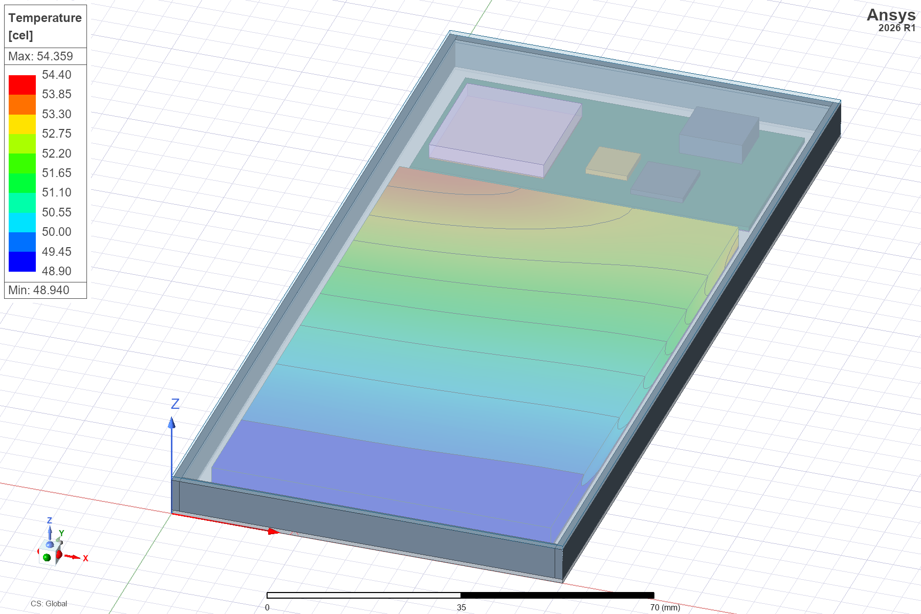
Inspect the corrected 5.5 W steady-conduction model: native battery, electronics and exterior contour views, selectable component statistics, mesh evidence and the original 15-page report.
Ansys IcepakSteady conduction671,368 cells
Illustrative assumptions · Saved volume maxima: battery 54.33 °C, processor 74.51 °C · Provisional results; heat balance, mesh independence and physical validation remain open. A separate model from the open-source stages.
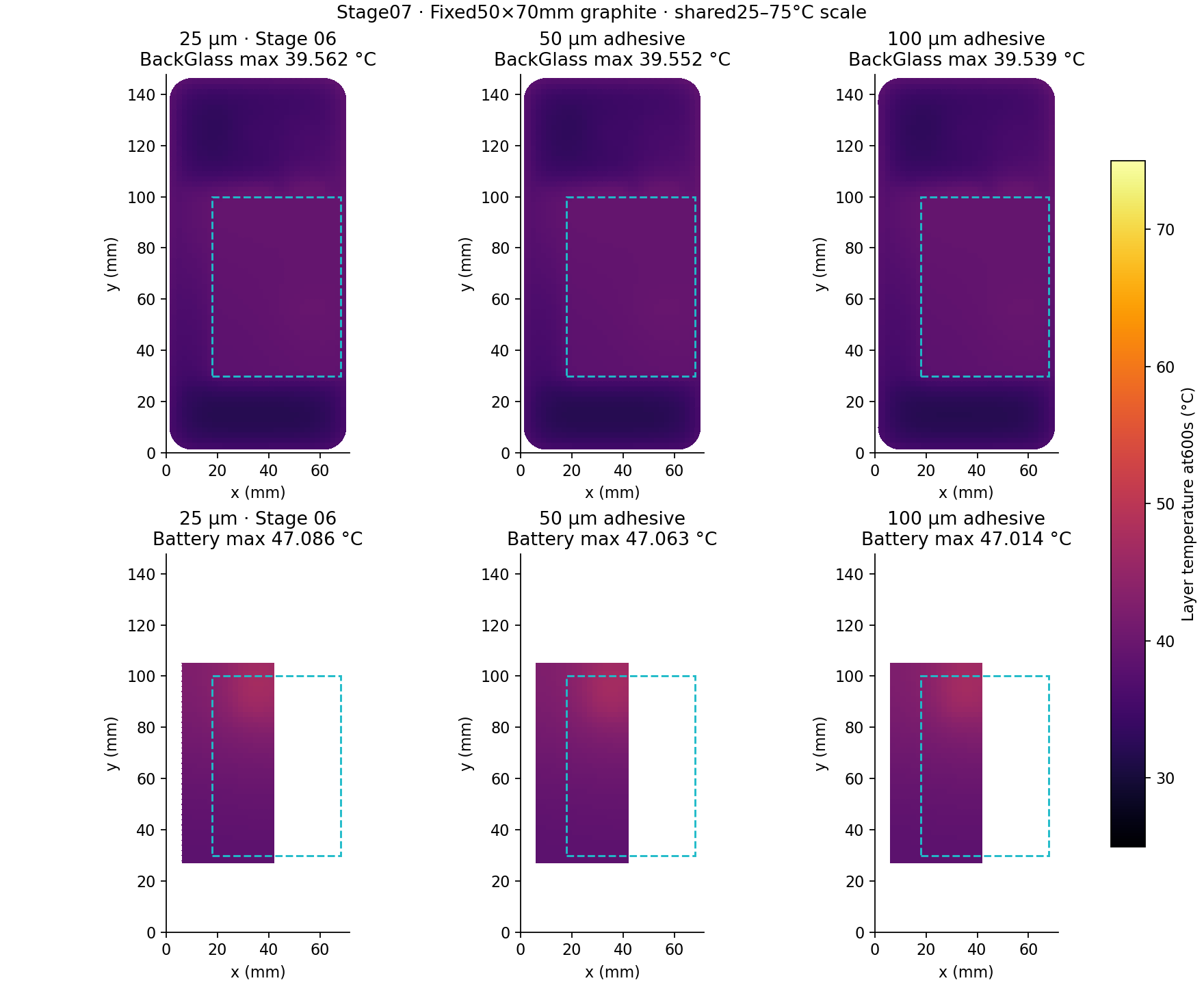
Start with one cell, then build a coupled PCB and enclosure model. The latest stage compares adhesive thicknesses under the largest graphite sheet, tracking cover and battery temperatures with a separate resistance-only diagnostic.
FreeCADPythonSciPyOpen source
Stages 01–07 available · Adhesive thickness and thermal coupling · Layered finite volumes and lumped packages · Assumed inputs · Numerically verified, not experimentally validated.
Explore an independent public-reference aircraft through a 0°–20° angle sweep and a full-domain transient wake study: native flow visualization, lift/drag loading, persistent circulation and fluctuating forces, with numerical limits documented.
Select an angle to pause and inspect. Use the video’s play control to resume the 0° → 20° → 0° loop. All eleven calculated angles remain on the plots; the highlighted point follows the displayed field. Use fullscreen for detailed plots on small screens.
Independent public-reference Archer Midnight approximation, presented with the Wisk methods demos. All eleven cases missed full convergence targets. This is an unpowered, symmetric screening study, not Wisk/Boeing/Archer engineering data or a validated stall envelope.
More details — full technical case studyFewer details — close technical case study
What the 0°–20° study shows
I extended the public-reference exterior reconstruction to eleven independent, unpowered calculations: 0°, 2°, 4°, 6°, 8°, 10°, 12°, 14°, 16°, 18° and 20° angle of attack at 100 mph. The stationary aircraft and camera make the changing inflow direction, surface loading and near-aircraft flow paths easier to compare. The native velocity and surface-traction fields come from OpenFOAM, while the three-second 0° → 20° → 0° sequence is an edited presentation of those fields.
The useful question is how increasing incidence changes the modeled lift/drag tradeoff and where the computed flow bends or reverses. The screening curve shows diminishing lift gains at higher angles and a strong drag increase. It identifies regions and angles for a better-resolved follow-up; it does not establish a production-aircraft performance curve, a stall angle, or a safe flight envelope.
This is an independent Khani Solutions demonstration built from public Archer Midnight photographs, exterior views and patent illustrations. It appears alongside the Wisk methods demos because it illustrates related engineering tools. Archer Midnight and Wisk’s aircraft are different designs. No employer or manufacturer geometry, operating data, proprietary battery details or flight-test results were used.
Surface colors: local signed lift or drag per unit area
The selectable colored variable is aerodynamic force contribution per surface area, in N/m² (equivalently Pa). It includes pressure and modeled viscous shear. It is neither surface pressure coefficient Cp, integrated lift/drag coefficient CL/CD, nor structural stress. A force density can have either sign: one patch can assist the selected load while another opposes it.
The incompressible OpenFOAM pressure is kinematic pressure pkin, in m²/s². With density ρ, outward normal of the fluid boundary nfluid, and OpenFOAM’s kinematic wall-shear vector τOF, the body traction used here is t = ρ pkin nfluid − ρ τOF. The installed OpenFOAM force and wall-shear conventions were checked before integration. The surface uses a zero-gauge reference; local pressure contributions depend on that reference, while a consistent closed-body pressure integral eliminates a uniform pressure offset.
Body X points from nose toward tail, Y spans the aircraft and Z points upward. At angle α, U∞ = V(cos α, 0, sin α), drag direction eD = (cos α, 0, sin α), and lift direction eL = (−sin α, 0, cos α). Colors show t·eL or t·eD. Native surface-cell tractions and areas are retained; cell-to-vertex averaging is used only for a smoother display. The common clipping ranges, ±1,800 Pa for lift and ±1,000 Pa for drag, allow comparison across angles. Saturated colors hide excursions beyond those display limits rather than limiting the calculated load.
The green lift and amber drag arrows share one length scale across all cases. They represent integrated wind-axis forces, with an illustrative drawing anchor. Their origin is not a calculated center of pressure or known aircraft center of gravity. The right-side plots contain all eleven case means; the highlighted point and vertical band track the displayed case. Whiskers show the minimum and maximum force within the declared iteration window, not confidence intervals or physical-time fluctuations.
Streamlines: calculated paths with presentation arrowheads
Cyan lines are selected paths through the native velocity field around the fuselage, above/below the wing and near the tail. Purple lines are selected near-body reverse-flow segments where the current solver iterate supports them. Curvature shows the calculated deflection of the flow. These lines are not a uniform sampling of the flow, and their count, spacing, brightness and thickness do not represent mass flow or boundary-layer thickness. A curling streamline in an unconverged steady field is a recirculation candidate, not proof of a resolved coherent vortex or a vortex-shedding frequency.
The body-fixed seed set used 90 wing releases distributed over 15 spanwise locations and six vertical offsets, 40 cabin releases at five lateral positions and eight heights, and eight tail releases. Each case could add up to 40 spatially separated seeds in near-body cells with reversed wind-axis velocity. Thus the main release positions are comparable across angles, while the wake seeds are selected from each case’s computed field.
PyVista/VTK traced paths bidirectionally using native U, an initial step of 0.025 m, minimum/maximum steps of 0.002/0.07 m, up to 3,000 steps, maximum length 16 m, terminal speed 0.15 m/s and integration-error tolerance 10⁻⁶. Cropping, minimum path length, velocity-deflection and spacing filters removed straight bypass paths and reduced overlap. At most five qualifying half-domain reverse-flow candidates were retained before mirroring. Selected full-aircraft path counts vary with angle; the 20° view contains 122 paths. No synthetic vortex curves were inserted.
Arrowheads point along interpolated U and move forward even when the displayed angle returns toward zero. Their speed is illustrative. The return branch reuses the same eleven steady fields; it is not an independently solved descending-angle sequence, a dynamic pitching maneuver, a hysteresis calculation, or three seconds of physical flow evolution. Matching opening/closing source images create the visual loop. The video is 1920 × 1080 at 24 fps; an eleven-second version allows slower inspection.
What the screening curve says
Between 12° and 16°, the mean modeled lift changes little: about 24.28, 24.47 and 24.41 kN, while mean drag rises from about 3.60 to 6.15 kN. At 20°, the mean lift is about 25.63 kN and drag about 8.69 kN. Relative to 12°, that is approximately 5.6% more lift and 142% more drag. The corresponding modeled L/D falls from about 6.75 to 2.95. These ratios describe this untrimmed, approximate, unconverged model; they are not predictions of the real aircraft’s cruise efficiency.
The engineering message is diminishing load benefit with a rapidly increasing drag cost in this particular screening sweep. The highest sampled mean lift occurs at 20°, but the data do not resolve a trustworthy lift maximum or establish a stall threshold. The negative lift at 0° belongs to the assumed symmetric-airfoil draft and its untrimmed orientation, not to an actual Midnight cruise condition.
AoA
Lift / kN
Drag / kN
CL
CD
Full convergence targets
0°
-1.349
1.272
-0.0483
0.0455
Not met
2°
+4.061
1.253
0.1454
0.0449
Not met
4°
+8.949
1.295
0.3204
0.0464
Not met
6°
+13.868
1.517
0.4966
0.0543
Not met
8°
+18.438
1.803
0.6602
0.0646
Not met
10°
+21.575
2.493
0.7725
0.0893
Not met
12°
+24.275
3.595
0.8692
0.1287
Not met
14°
+24.466
4.886
0.8760
0.1750
Not met
16°
+24.409
6.150
0.8740
0.2202
Not met
18°
+25.559
7.228
0.9152
0.2588
Not met
20°
+25.632
8.689
0.9178
0.3111
Not met
Forces are full-aircraft equivalents: the symmetry-half integral is doubled. Coefficients use the matching half reference area, 11.407946 m²; full reference area is 22.815892 m² from the assumed draft chord distribution. The plots use the last 200 second-order SIMPLE iterations, while colors and streamlines use the final steady iterate. A field integral should therefore be compared with the native final force, not automatically with the iteration-window mean.
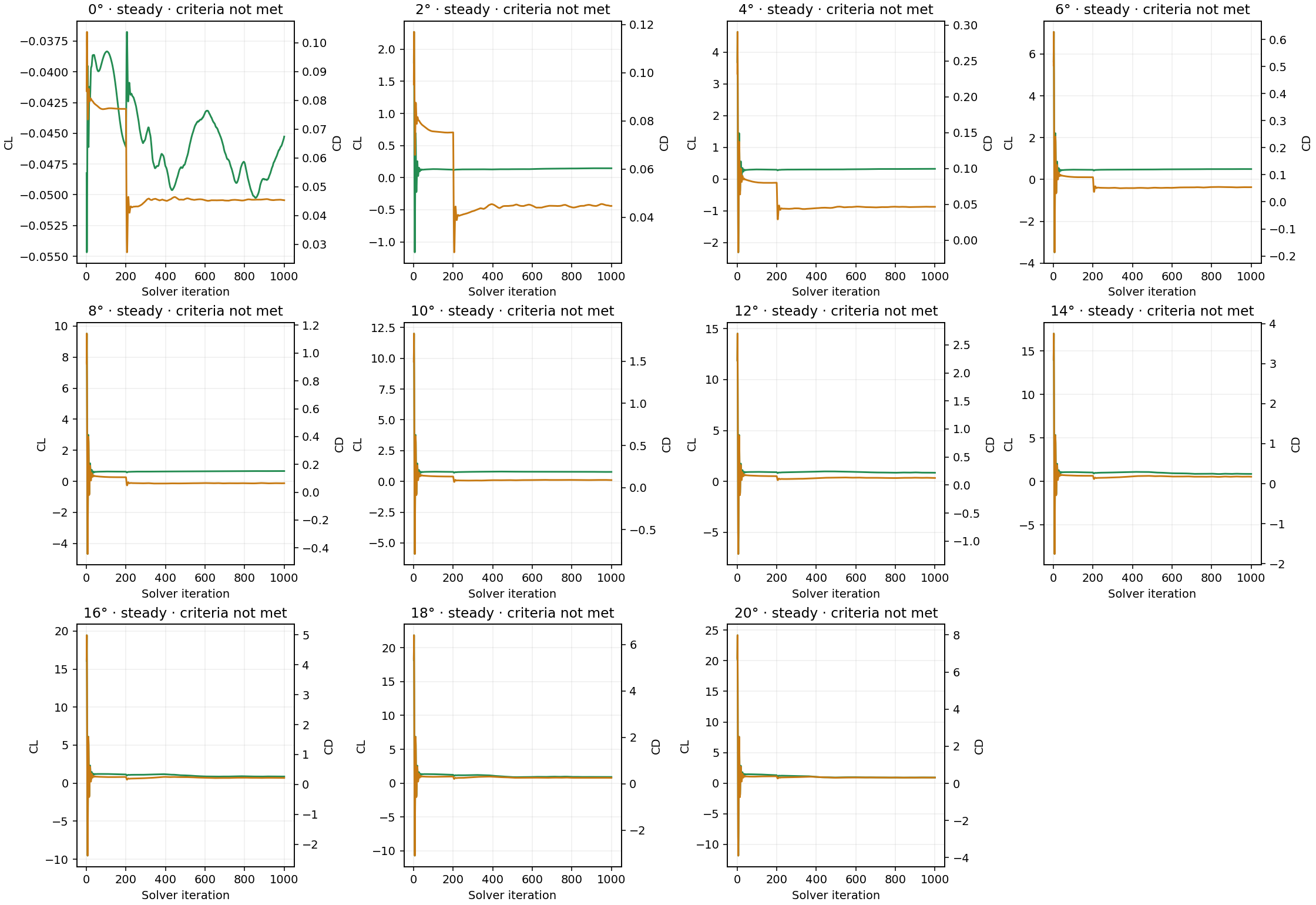
Retained force/residual history evidence. Every case missed the full convergence targets, even though its global mass-balance check passed.
What to investigate next
Examine wing/cabin-root transitions, nacelle/boom junctions, exposed gear and the tail in fixed views at the same operating point. Surface traction maps show which patches contribute positively or negatively to a force; velocity paths show where the current field is deflected or reversed. A useful design change still needs a controlled geometry comparison with converged, mesh-sensitive loads. These movies do not demonstrate a fairing benefit or an optimized aircraft.
Priority follow-up is to establish representative airfoil, incidence and twist; improve near-wall resolution and mesh conditioning; resolve the nonlinear force histories; and compare systematically refined grids. High-angle separated flow may require a sufficiently long, time-resolved calculation, timestep sensitivity and statistical averaging. Lift/trim and pitching-moment interpretation require a justified CG and control settings. Rotor interactions require a justified powered representation. Those tasks were not completed by extending the visual angle sweep.
CAD preparation and the high-angle volume mesh
The editable Blender 5.0.1 exterior was reconstructed from multiple public views using a visually fitted fuselage loft, glazing patches, landing-gear fairings, wing-root shoulders, six booms, cruise-oriented forward nacelles/hubs and a V-tail. The main wing uses a generic symmetric 13%-thickness profile; the tail uses a generic 10%-thickness profile. OEM camber, incidence, twist, control settings, trim and structural shape were unavailable. The earlier CAD section below documents scale references and reconstruction assumptions.
The CFD exterior is a separate cleaned body: propeller blades and decorative surface patches were omitted; cabin closure, wings, tail, booms, nacelles/hubs and exposed gear remain. A 25 mm voxel union, smoothing and triangulation produced a connected closed boundary, with approximate component tags. These operations round thin trailing edges and small details. A visually convincing, watertight surface is not evidence of aerodynamic fidelity.
The high-angle study uses a new common 2,226,297-cell symmetry-half mesh for all eleven cases, not the earlier 474,386/1,210,614-cell baseline grids. OpenFOAM v2512 blockMesh and snappyHexMesh refined the wing, tail and nacelle surfaces to level 7 and the other aircraft surfaces to level 6. The near-body box uses level-3 refinement; the refined wake was expanded to X = 0–30 m, Y = 0–10 m and Z = −3–16 m to cover high-incidence flow. The full external half-domain spans X = −35–75 m, Y = 0–35 m and Z = −30–35 m, with symmetry at Y = 0.
Layered meshes and a local cell-splitting repair were tested and rejected because of poor stencil quality. The accepted surface-refined mesh has no extruded prism layers and uses wall-function RANS. This improved the chosen mesh-quality diagnostics but did not establish adequate boundary-layer profiles or skin-friction accuracy. Fifteen tiny deficient fluid cells were closed in three passes (9, 5 and 1); total removed volume has an upper bound of 0.00015 m³. Their new walls were assigned to the nearest existing aircraft patch. The rejected attempts and native audit logs remain in the engineering archive.
Configured mesh checks passed. Expanded audits reported no weak-determinant cells or low-weight faces at the retained criteria; minimum normalized determinant was 0.0011844321 and minimum face weight 0.087647394. The expanded concave-cell diagnostic still failed, identifying 81,478 cells. Thus this is not an “all checks passed” mesh, and it is not grid independent. A mesh fingerprint confirmed that every angle used the same points, faces, ownership, neighbor and boundary files.
Solver settings, execution and acceptance
The computations ran on the Intel Xeon Gold 6238R machine. Meshing used 16 MPI ranks. Each angle used four MPI ranks, with eleven cases scheduled concurrently and an aggregate cap of 44 ranks. The method was OpenFOAM v2512 simpleFoam: steady incompressible RANS with k–ω SST, not a Blender fluid simulation. Blender preserves editable geometry and field attributes; Python, NumPy, PyVista/VTK, Pillow and FFmpeg produced the native-field visualization and H.264 videos.
1,000 steady iterations; final 200 second-order iterations for means and ranges
Equation-residual targets
Final initial p residual ≤ 10⁻⁴; U, k and ω ≤ 10⁻⁵
Force-window / mass targets
Cd relative peak-to-peak range ≤ 1%; Cl absolute range ≤ 0.002; relative net boundary volume flux ≤ 10⁻⁴
Outer boundaries impose the prescribed freestream direction with compatible pressure/freestream treatment; the aircraft is no-slip with zero-gradient pressure and SST wall functions. The archived settings file contains the actual 0° and 20° boundary dictionaries, discretization and SIMPLE controls. At 20°, U∞ ≈ (42.008, 0, 15.2897) m/s, eD = (0.939693, 0, 0.342020), and eL = (−0.342020, 0, 0.939693).
All eleven solves ended normally at their bounded run limit, but none met every declared residual and force-window target. All mass-balance checks passed. Global flux closure and successful process exit do not establish momentum convergence, a stable force curve, a correct separation pattern, or physical validation. SIMPLE “time” in these records is an iteration counter rather than seconds.
Short pimpleFoam SST URANS trials were initialized from the steady fields, with backward time discretization, two outer corrections, one pressure correction, one non-orthogonal correction, adaptive timestep and maximum Courant number 1. Their measured timestep cost would have required hours to reach useful averaging. They were ended cleanly before the intended 0.03 s averaging start. These short trials produced no usable unsteady mean; every field in the angle-sweep movie is a steady screening iterate. The separate full-domain transient follow-up above subsequently reached approximately 2 s and reports its own statistics and limitations. The short-trial record gives actual termination times and does not treat the video duration as simulated time.
Independent surface pressure/shear integration was cross-checked against native final OpenFOAM forces to verify signs, area mapping and projection. Pressure and viscous integral discrepancies were at most about 0.0362% across the recorded checks. Agreement between two calculations from the same iterate checks post-processing consistency; it does not validate that iterate’s physical accuracy. Coefficient/force normalization and component-force sums were also checked.
Symmetry excludes asymmetric stall modes. No propeller blades, thrust, propwash, resolved rotor wakes, ground effect, internal cooling, trim, structural loads or aeroelastic response were solved. No grid or timestep independence, flight-test correlation, OEM validation, or reliable maximum angle of attack has been established.
Inspect the evidence and editable visualization
The Blender source contains one common stationary mesh, 22 per-vertex scalar attributes (lift and drag for eleven angles), native streamline geometry and wind-axis force arrows. Scene controls CaseIndex = 0…10 and ColorMode = 0/1 select the field and lift/drag coloring. The updated 72-frame timeline sweeps 0° → 20° → 0°. Reopening and every frame’s case/visibility selection were verified on Intel. The final composite movie is rendered with PyVista/VTK; the Blender file is an editable scientific visualization, not a separate CFD solver.
Public portfolio update: October 14, 2026. Numerical values in this steady-sweep section refer to the common-mesh high-angle screening study. Original native volume fields, logs, rejected meshes and execution records remain in the engineering archive.
A reconstructed aircraft center section and a prescribed hot-gas pulse show how exhaust interacts with the fuselage and ground, spreads, and disperses after venting stops.
More details — full technical case studyFewer details — close technical case study
The engineering challenge
Routing battery vent gas outside an aircraft is only part of the problem. Once a hot jet leaves the outlet, its momentum, buoyancy, the fuselage shape, and the nearby ground determine where it travels. A downward-facing vent can move the initial release away from the cabin yet create a hot region below the aircraft. The plume can spread along the ground, entrain surrounding air, and turn upward as it loses momentum.
I built this external-flow study to make those interactions visible for a stationary aircraft on the ground. The purpose is to establish a repeatable geometry-to-results workflow for examining a hypothetical thermal-runaway exhaust release. The model helps frame questions about outlet placement, clearance, local recirculation, and the persistence of hot gas after venting stops.
This is an independent Khani Solutions portfolio demonstration using an approximate Archer Midnight-inspired body reconstructed from public images. The outlet and release conditions are my assumptions. It is not an Archer or Wisk design analysis, employer project, certification result, or assessment of either company's battery safety.
What was modeled
The calculation resolves only the air outside a vertical, longitudinal aircraft center section. A prescribed hot-gas boundary represents exhaust that has already left the battery system. Cell failure, pack pressure, gas generation, propagation, and the internal vent duct are not solved. Consequently, the simulation predicts external flow and gas temperature for the specified release; it does not predict whether thermal runaway occurs or what a real pack would discharge.
Thermal-runaway exhaust can involve composition changes, combustible gases and particles. Here it is represented as a single nonreacting, air-like gas. The colored field is gas temperature, rather than a species concentration, flame, smoke-density field, or toxic-exposure measure.
Step 1 — Reconstruct and review the center section
I compared public side, front three-quarter, rear three-quarter, and elevated views of the black Midnight aircraft. An early side outline included features that lie outside the center plane. I replaced it with an estimated three-dimensional fuselage envelope built from 17 cross-sectional stations in FreeCAD, then intersected that envelope at the lateral coordinate y = 0. This produces a nose-to-tail center cut rather than using the entire projected side silhouette as a solid CFD obstruction.
The estimated fuselage is 7.2 m long. Image scaling uses an assumed 8.2 m projected whole-aircraft nose-to-tail-tip extent. Those dimensions, hidden contours, cross-sectional widths, and an assumed centered nose fairing are reconstruction inputs, not manufacturer measurements. The wing attachment is blended into the roof estimate. Off-center main landing-gear fairings, wing and rotor booms, and V-tail arms are excluded from the solved plane.
I overlaid the center cut on the reference image and reviewed the estimated envelope from multiple views before meshing. The approved 25 mm clearance beneath the assumed nose fairing was retained; the model does not establish actual tire contact. CAD validity, section planarity, and the exposed 100 mm vent edge were checked. The native FreeCAD and STEP geometry uses millimetres; the CFD geometry uses metres.
Step 2 — Define a hypothetical ground release
Scenario inputs — assumptions rather than measured aircraft data
Input
Value used
Aircraft and rotors
Stationary, on the ground; rotors stopped
Ambient
Still air at 25°C; hydrostatic pressure referenced to 101,325 Pa at ground level
Gravity
9.81 m/s² downward
Outlet
100 mm flush belly slot, centered at longitudinal x ≈ 4.9000 m and height ≈ 0.7004 m; x increases from nose toward tail
Exhaust temperature
600°C (873.15 K)
Jet velocity
40 m/s, directed 35° aft and downward; components (32.7661, −22.9431, 0) m/s in solver coordinates
Release timing
0–10 s venting, then a closed no-slip adiabatic mouth and 5 s additional dispersion
Walls and ground
Stationary, no slip, adiabatic
External domain
Longitudinal x = −16.4 to 32.8 m; height = 0 to 24.6 m
2D representation
One cell through a 0.1 m extrusion; front/back boundaries are empty
The prescribed release is an illustrative pulse. Closing the mouth at 10 s is also an assumed scenario, not a model of a real vent valve. A 2D slot represents flow per unit span; it is not a 100 mm diameter nozzle. Normal mass flux depends on the local slot normal as well as jet direction, so this case is not a controlled mass-flow comparison with the earlier protruding-outlet concept.
Step 3 — Generate and check the external-fluid mesh
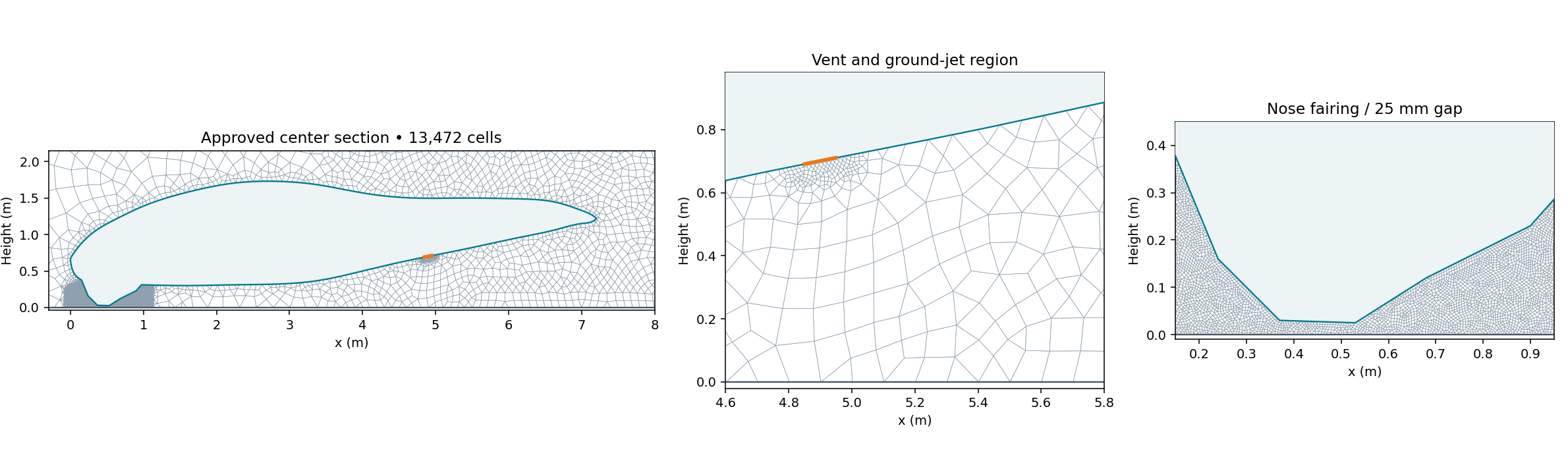
Gmsh 4.15.2 generated the external-air mesh around the approved section. The wall was simplified to remove very short construction segments while preserving the vent endpoints. Maximum boundary deviation from the CAD cut was approximately 0.952 mm. The mesh contains 13,472 finite-volume cells and eight faces across the outlet, with a single cell through the span.
Target sizes were 12.5 mm near the vent, 6 mm around the nose-fairing gap, approximately 80 mm near the body, 100 mm in the near-ground release zone, 230 mm in the wider plume region, and up to 1.5 m in the far field. The local targets focus resolution on the source, clearances, and initial ground interaction. No dedicated wall-normal boundary-layer stack was established; wall functions were used, and wall-resolution independence was not demonstrated.
OpenFOAM's checkMesh -allTopology -allGeometry returned Mesh OK. Maximum non-orthogonality was 44.54° and maximum skewness was 1.57. These checks support a usable numerical mesh; they do not establish grid-independent plume temperatures.
Native external-fluid mesh and local detail around the outlet and nose gap.
Step 4 — Set up the flow and thermal solver
I used OpenCFD OpenFOAM v2506 buoyantPimpleFoam for transient compressible, buoyant, nonreacting flow with sensible-enthalpy transport. Density follows the perfect-gas equation of state, allowing the hot exhaust to be less dense than ambient air. The gas molecular weight is 28.965 kg/kmol, with constant specific heat Cp = 1,005 J/(kg·K). Sutherland viscosity uses As = 1.458 × 10⁻⁶ and Ts = 110.4 K. This is an air-property approximation across the imposed temperature range.
Turbulence is modeled using RANS k–omega SST. At the release boundary, k = 6 m²/s² and omega = 638.9 s⁻¹; initial ambient values are k = 10⁻⁶ m²/s² and omega = 1 s⁻¹. Aircraft and ground use kqRWallFunction, omegaWallFunction, nutkWallFunction, and the compressible thermal wall function. Turbulence closure and the 2D assumption influence entrainment and vortex behavior.
The aircraft and ground impose zero velocity and zero temperature gradient. The outer boundary uses pressureInletOutletVelocity, inletOutlet temperature with 25°C on inflow, and prghTotalPressure with a hydrostatically initialized pressure profile. Fixed-flux pressure conditions are used on walls and the mouth. The initial field is hydrostatic, rather than uniform pressure under gravity.
Numerical settings from the completed native case
Setting
Configuration
Time integration
First-order implicit Euler
Convection
Gauss upwind for velocity, enthalpy, kinetic energy, k and omega
Gradients / diffusion
Cell-limited Gauss linear gradients; Gauss linear limited 0.5 Laplacian; limited 0.5 normal gradients
PIMPLE coupling
Momentum predictor enabled; one outer corrector, two pressure correctors, zero non-orthogonal correctors
PBiCGStab with DILU; absolute tolerance 10⁻⁷, relative tolerance 0.05; final relative tolerance 0
Density solution
PCG with DIC; absolute tolerance 10⁻¹⁰, relative tolerance 0
Time-step control
Initial step 10⁻⁵ s; adaptive stepping; maximum step 0.002 s; maximum Courant 0.6 at startup and 0.8 during continuation
Saved fields
Every 0.25 s; 61 native snapshots including 0 and 15 s
Compute
Local ARM64 Docker OpenFOAM runtime; six MPI ranks after serial startup, Scotch decomposition
First-order schemes provide a robust starting point but introduce numerical diffusion. Residual tolerances specify the linear solves; they are not measures of physical prediction accuracy.
Step 5 — Run startup, release, and dispersion
Before injecting hot gas, I ran an independent 0.25 s quiet-atmosphere check. Its maximum speed was 0.000221 m/s, indicating that hydrostatic initialization did not create a substantial artificial background flow. The release calculation then ran serially to 0.25 s, followed by a six-rank pilot to 0.5 s and continuation to 10 s. At that point the mouth was converted to a closed wall, and the calculation continued to 15 s.
Both the release and dispersion phases ended normally. Every saved temperature, velocity, pressure, and density field was checked for finite values, with positive pressure and density and accepted temperature bounds. Inlet mass flux, outer-boundary mass flux, and total fluid mass were monitored every solver timestep, producing 124,652 samples. The largest monitored step was approximately 0.000963 s.
Step 6 — Audit mass balance and interpret the results
The imposed jet initially carries hot gas aft and toward the ground. The evolving velocity field shows ground interaction, spreading and recirculation, while buoyancy and entrainment alter the plume as it slows. After source closure, the nearby temperature field decreases as hot gas mixes and moves away. The video shows these calculated processes for this particular pulse, geometry, and still-air scenario.
Results from the completed 0–15 s run
Quantity
Calculated value and interpretation
Injected mass
1.168359 kg for the modeled 0.1 m span over 10 s; average inlet flow 0.116836 kg/s for that span, or 1.168359 kg/s per metre of slot span
Peak saved external-cell temperature
598.61°C, close to the imposed 600°C source
Peak monitored gas temperature adjacent to ground
222.67°C; gas at an adiabatic fluid boundary, not ground-material temperature
Maximum saved cell speed
44.72 m/s
Maximum cell temperature at 15 s
65.77°C, five seconds after the release stops
Maximum near-ground cell temperature at 15 s
47.08°C; a separate cell-based metric from the boundary monitor
Maximum cell speed at 15 s
4.52 m/s
Area above 60°C at 15 s
0.429 m² in the modeled section; not a 3D exposure volume or safety zone
Maximum mass-inventory residual
0.000191 kg, or 0.01636% of injected mass, using every-step monitors and Euler end-step flux integration
Independent saved-field mass audit
Maximum residual 0.00533% of injected mass; final saved-field inventory differs from the function-object monitor by 0.000126 kg
The mass audit compares domain inventory change with injected mass and net outer-boundary mass flow. It includes ambient inflow and outflow, not just the hot release. The small difference between saved-field and function-object inventory is recorded separately; its precise update-order cause has not been traced. Good mass closure is a numerical consistency check, not experimental validation.
The peak ground-adjacent gas value identifies a location worth studying further. Because the solid ground and aircraft heat conduction are absent, it cannot establish skin temperature, ground heating, thermal damage, or acceptable human exposure. The final temperature decrease is specific to this short pulse and open domain; it should not be generalized to a longer pack release.
Step 7 — Create a readable scientific video
I rendered the native temperature and velocity results into a 10-second, 1600 × 900 H.264 video at 30 fps. The 15 physical seconds play at 1.5× speed. A white background, Turbo scale from 30–600°C, and dark instantaneous streamlines keep the flow visible. Gas below 30°C is white, and 30–40°C blends into white. Spatial and temporal interpolation smooth the display; reported numerical metrics use native fields.
The fixed view covers longitudinal x = −3 to 14 m and height −0.1 to 8 m. Plume outside that window is cropped from the video but remains part of the CFD domain. The nose points right for agreement with the reference. Streamlines describe the instantaneous velocity field; they are not trajectories of tracked gas particles.
The pencil aircraft overlay is an AI-assisted visual derived from the public side reference and aligned using a uniform scale and landmarks. It supplies recognizable aircraft context. Off-center gear, booms, and tail features visible in the sketch are not CFD obstacles. The approved center-cut boundary remains the solved wall. Image generation supplied the presentation overlay only; temperature and velocity come from OpenFOAM. Plain-section and photo-based variants were also made, and all three videos were fully decoded and checked for their 300 frames and 10-second duration.
How this helps engineering decisions
A workflow like this can support early comparisons of vent location, direction, release history, aircraft clearance, ambient wind, and surrounding obstacles. It can help choose where to place thermocouples and flow diagnostics in a later physical test, or identify regions needing a coupled solid-heating model. Those comparisons have not been run here; this study establishes one screening case and its audit trail.
For design use, the next steps are measured time-dependent mass flow, temperature, composition and pressure; verified aircraft and vent geometry; three-dimensional flow; mesh, time-step and domain studies; turbulence and wind sensitivity; and comparison with a representative release experiment. Chemistry, radiation, particles, species transport, rotor flow, and solid conduction should be added where the engineering question requires them. Exposure limits, thermal-damage limits and evacuation distances require additional evidence.
The battery cooling study elsewhere in this portfolio addresses a different question: how generated heat moves through a module and its coolant circuit during an imposed operating load. The plume study starts at an assumed external vent source. Neither demonstration predicts cell failure or thermal-runaway propagation, and they are not coupled simulations.
Case identifier: midnight-ground-tr-r5, completed October 11, 2026. The local engineering archive retains the approved FreeCAD/STEP section, geometry assumptions, Gmsh definition, native OpenFOAM dictionaries and fields, complete phase logs, every-step mass monitors, analysis scripts, overlay provenance and video checks. The public site provides the numerical run summary and the solver settings. Full native case files remain in the engineering archive.
A 30-cell equivalent module, titanium casing, and two liquid cold plates in series show how internal thermal resistance and coolant warming affect transient cooling.
More details — full technical case studyFewer details — close technical case study
The challenge and why simulate it
Battery cooling must move heat from the module interior through interfaces and into the coolant. Low through-plane conductivity, local heat generation, cold-plate coverage and coolant warming can produce temperature differences that a single bulk-temperature estimate misses.
I built this independent thermal screening example to examine a series cooling architecture: two cold plates cool opposite faces, while the second plate receives water already warmed by the first. It illustrates why coolant temperature alone does not establish the hottest module temperature, and why transient heat storage must be included when interpreting cooling performance.
This is a Khani Solutions portfolio demonstration using assumed materials and operating conditions. It is not proprietary Wisk or Boeing hardware, an employer analysis, or a validated aircraft battery design. It is an operating-load cooling model, not a thermal-runaway initiation, propagation or exhaust calculation.
Workflow, model and results
I built this conjugate heat transfer study using FreeCAD for the geometry and Elmer for the flow and thermal calculations.
The model represents 30 pouch cells as a single anisotropic thermal block, measuring 352 × 188 × 169 mm, inside a 2 mm titanium casing. Two aluminum cold plates sit on opposite faces, separated from the casing by 0.5 mm thermal interface layers. Each plate contains a five-pass serpentine channel. Coolant passes through the first plate, crosses to the second, and then exits.
The battery conductivity was assumed to be 20 W/m·K in-plane and 1 W/m·K through-plane. That difference matters: a cold plate can remain relatively cool while the module interior heats up because heat cannot reach the cooled faces quickly enough.
The simulation used:
300 W of uniform module heat generation.
1 L/min water at 25°C, with all regions initially at 25°C.
Approximately 2.08 million tetrahedral elements.
A steady incompressible flow calculation followed by transient conduction and coolant advection, using 30-second steps over one hour.
At one hour, the calculated module peak reached 63.5°C, while the coolant reached 26.4°C after the first plate and 27.8°C at the outlet. The coolant was removing approximately 195 W at that instant; the remaining heat was still accumulating in the assembly. This was a transient result, not thermal equilibrium.
Practical design concerns include warmer coolant entering the second plate, pressure losses through both serpentine circuits, insufficient pump flow, channel blockage, and thermal interface gaps or uneven compression. The interfaces here were perfectly bonded; those defects were not simulated.
This is an illustrative screening study. The flow regime is transitional, although modeled as laminar. A mass-conserving flux reconstruction changed the calculated velocity field by about 22%, so flow refinement, turbulence sensitivity, mesh/time-step studies, and experimental comparison are needed before using these temperatures for design decisions.
The video compresses one simulated hour into 10 seconds.
What to do with these results
Use this example to frame architecture and test questions: whether a parallel coolant arrangement changes temperature uniformity, how flow rate affects heat removal and pumping demand, and how interface resistance or cell-to-cell heat variation affects the hotspot. Those variations and defects were not calculated in this run. The imposed 300 W load remains an input, rather than a prediction of electrochemical heat generation.
Design qualification would require representative material and interface measurements, adequate flow resolution, turbulence sensitivity where appropriate, mesh and time-step convergence, and comparison with module and circuit test data. A relatively cool outlet is not proof of a cool module core. A one-hour transient result is not a demonstrated steady operating limit.
Connection to the external plume study
Cooling and venting belong to different parts of battery thermal engineering. This model follows heat conduction and coolant transport in a module assembly. The aircraft plume study follows a hypothetical external hot-gas source after discharge. The two demonstrations share a focus on thermal-fluid behavior but are not coupled and do not establish thermal-runaway prevention.
An editable Falcon 9-inspired assembly connects exterior aerodynamics, wall heat transfer, multiphase tank pressurization and diffuser hardware through one documented public-data geometry foundation.
Blender 5.0.1PythonPublic references
CAD and film complete · Aerodynamic, tank and diffuser CFD planned.
Independent Khani Solutions work. Related to cryogenic methods in the Blue Origin experience section; not Blue Origin hardware or a manufacturer model.
A moving mesh follows wave propagation and the evolving free surface. Motion settings and absorption zones help control deformation and reflected waves.
Mission gas budgets and transient cryogenic subsystem analysis at Blue Origin; battery cooling architecture, pressure drop, and coolant distribution at Boeing / Wisk.