 Khani Solutions
Independent open-source thermal study
Double the heat input.
Stage 02 compares the same cell at 1 W and 2 W. A separate spatial extension shows how concentrating that same 2 W can produce a local hot spot.
All inputs are illustrative assumptions. These are numerically verified teaching models, without experimental validation. The spatial solve includes the effective pouch cell only; the surrounding CAD components have no calculated temperatures yet.
1 W versus 2 W: one change at a time
The cell geometry, thermal capacity, cooling coefficient, 25 °C ambient and timing are unchanged. Both sources run for 10 minutes, followed by 20 minutes of cooling. These wattages are prescribed heat generation, not electrical charging input power.
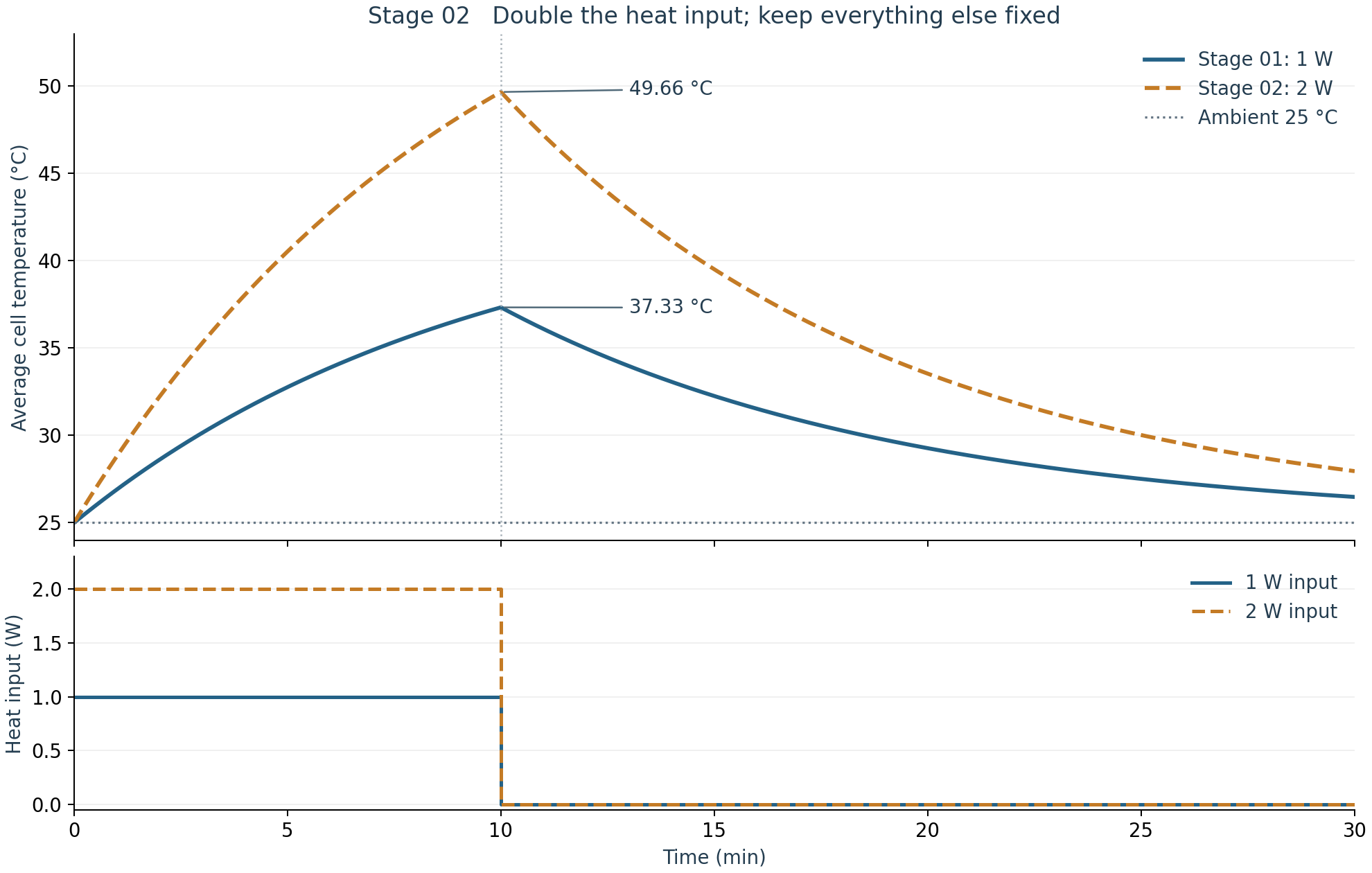
| Measure | Stage 01 · 1 W | Stage 02 · 2 W |
|---|---|---|
| Peak at 10 min | 37.33 °C | 49.66 °C |
| Rise above 25 °C ambient | 12.33 K | 24.66 K |
| Temperature at 30 min | 26.48 °C | 27.95 °C |
| Total heat supplied | 600 J | 1200 J |
Why the temperature changes
C · dθ/dt = Q̇ − G · θ with θ = T − Tambient
With constant thermal capacity C and conductance G, doubling Q̇ doubles the temperature rise above ambient. At heat-off the rises are 12.33 K and 24.66 K. The 2 W temperature is therefore 25 + 24.66 = 49.66 °C; the Celsius temperature itself does not double.
The larger temperature difference also doubles the instantaneous heat loss to ambient. Both cases retain the same time constant, τ = C/G: after heat-off they shed the same fraction of their excess temperature over a given time, while the 2 W case remains hotter. Nonlinear radiation, temperature-dependent properties, or electrical feedback would change this exact scaling.
Temperature maps on the cell and context CAD
Choose either average-temperature case or a spatial case, then move through time. The 2D spatial model uses 1,248 finite-volume cells and resolves in-plane temperature differences. Its field is displayed through the CAD cell’s thickness, matching the thin-cell assumption.
Loading solved temperatures and CAD…
Drag to rotate · Scroll to zoom · Temperatures apply only to the cell
How to read the spatial map
The uniform-source spatial control spreads 2 W over the cell. The localized example puts 80% of the same total 2 W into an assumed 12 × 18 mm region; the other 20% is spread throughout the cell. It adds no extra power. In-plane conductivity is assumed to be 20 W/(m·K).
The localized case has an average of 49.64 °C at 10 minutes but a 59.15 °C peak; the uniform-source spatial control peaks at 49.75 °C. Heat must conduct away from the concentrated source, so local temperature can rise substantially above the average. These source and material assumptions are not measurements of a product or a fault.
The shared scale stays at 25–65 °C across all cases and times. Focused mode changes the color range for the current frame; read the numerical endpoints before comparing colors. Surface colors are interpolated from finite-volume cell-center temperatures. No through-thickness gradient is solved, and gray phone components are geometry context only.
Static temperature maps at 10 minutes
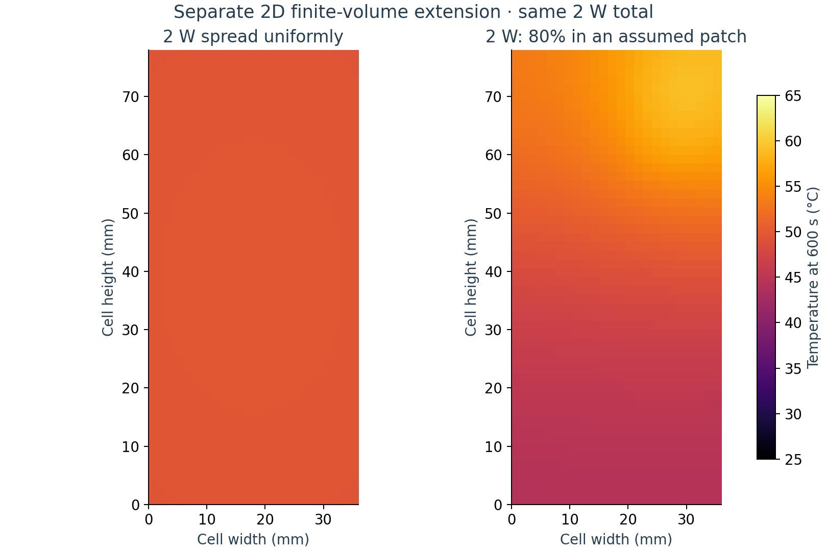
These are the two spatial cases, both at 2 W total input. The fixed scale matches the viewer's shared scale.
Spatial method, mesh and verification
The finite-volume model balances stored energy, neighboring-cell conduction, the prescribed heat source, and effective surface losses. Both broad faces and four edges use the same 8 W/(m²·K) effective loss coefficient as the lumped comparison. Edge faces include half-cell conduction resistance. The cell remains uncoupled from the enclosure and electronics.
Ci · dθi/dt = Q̇i − Σ Gij(θi − θj) − Gloss,iθi
- Thermal grid: 24 × 52 quadrilateral cells, 1.5 mm spacing; 1,325 corner points.
- Time integration: Crank–Nicolson with 0.5 s steps and sparse LU factorization in SciPy. Source-off occurs exactly at 600 s.
- Numerical checks: analytical limiting case, energy balance, 1,248 versus 4,992 cells, and 0.5 versus 1.0 s time steps. Refining the grid changed the localized peak by 0.00846 K; changing the time step changed it by 0.00000277 K. Full checks are in the verification JSON.
- Saved fields: browser frames every 10 s; ParaView-compatible PVD/VTU fields every 60 s for both spatial cases.
The mesh shown on the CAD cell is the 2D planar thermal grid. It is not a 3D assembly mesh. Stage 03 adds a separate coupled solution for the cell, PCB, packages and enclosure. The Stage 02 fields above remain cell-only.
Reproduce and inspect the results
All calculations use free and open-source Python, NumPy, SciPy and Matplotlib. Open the PVD files from the VTK archive in ParaView to inspect the time-dependent spatial results.
Method references: SciPy sparse factorization · Lumped and spatial thermal model hierarchy. The spatial solver here is custom finite-volume code; it does not run PyBaMM.