Independent parallel workflow · Ansys IcepakExplore the corrected Icepak PCB results
A separate illustrative smartphone assembly with native contour views, saved component maxima and vertex averages, mesh and solver evidence, and downloadable report and project files. Its inputs differ from these open-source stages, so this is not a matched solver benchmark.
Open the interactive Icepak study → Report & downloads →
KHANI SOLUTIONS · INDEPENDENT OPEN SOURCE STUDYBattery thermal modeling
Stage 01 — One cell, one temperature
We start with the energy balance for a pouch-cell equivalent. A prescribed heat source warms the cell; heat transfer to the surroundings cools it. Every additional stage will answer one new question.
All material and boundary-condition values are teaching assumptions. This is a solved, numerically verified model; it has no experimental validation and predicts no Apple or Wisk product performance.
Average temperature at the selected time25.00 °C
Uniform color represents the single temperature of this 0D model. It is not a spatial temperature contour.
Heat input: 1.0 W
The model in one equation
C · dT/dt = Q̇in − G · (T − Tambient)
C is the cell's thermal capacity in J/K. G is the effective conductance to ambient in W/K. The temperature rises when heat input exceeds the heat transferred out.
29.99thermal capacity, J/K
18.85thermal resistance, K/W
9.42time constant, min
The prescribed source is 1 W of heat. It is not 1 W of electrical charging power. We will calculate electrical-to-thermal conversion in a later stage.
0.0heat supplied, J
0.0energy stored, J
0.0heat transferred out, J
Heating and cooling result
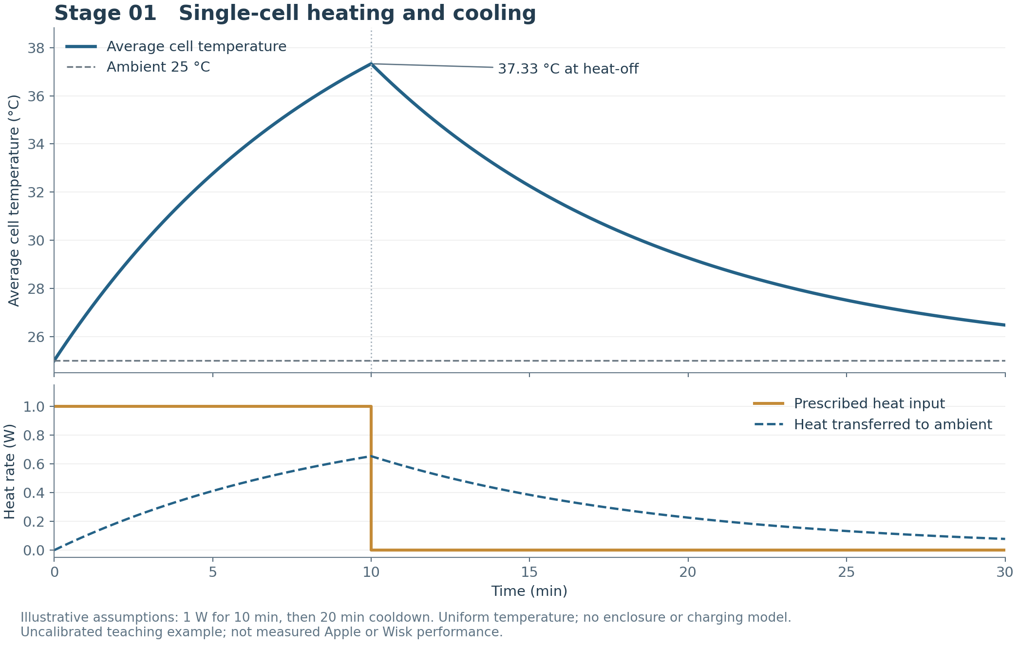
With these inputs, the average temperature reaches 37.33 °C at 10 minutes and falls to 26.48 °C at 30 minutes. The temperature stays continuous when the heat source switches off; its slope changes.
Energy is conserved
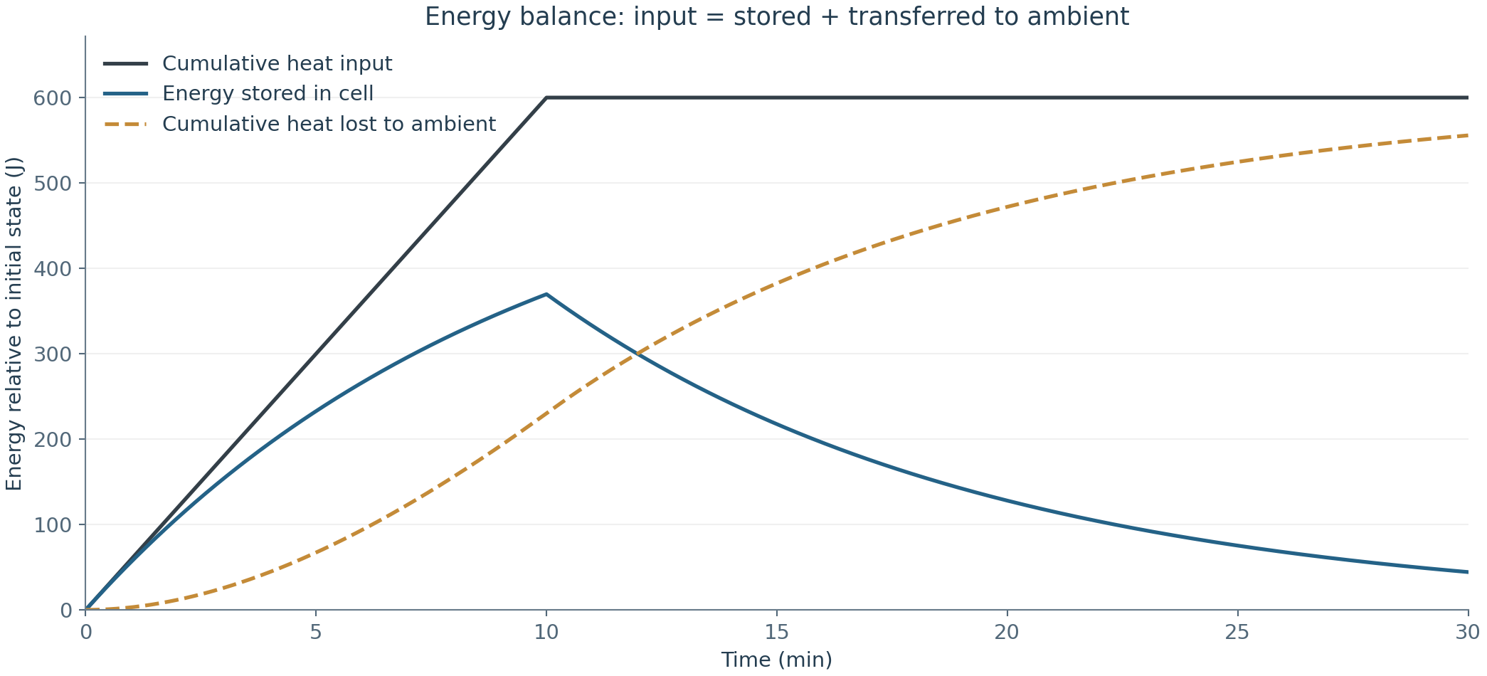
The source supplies 600 J in total. At each time, that energy is split between energy stored above the initial temperature and cumulative heat transferred to the surroundings. The maximum computed balance residual is 1.02e-12 J. Numerical and analytical temperatures agree within 3.43e-10 K; this verifies the implementation for these assumptions.
Inputs you can inspect
| Input | Value | Meaning |
|---|
| Cell envelope | 36 × 78 × 4.45 mm | Assumed equivalent rectangular cell |
| Density / specific heat | 2400 kg/m³ / 1000 J/(kg·K) | Assumed; not supplier measurements |
| Derived mass / exposed area | 29.99 g / 0.0066306 m² | Computed from the envelope and density |
| Effective surface loss | 8 W/(m²·K) | Same coefficient on all six faces; linearized combined loss |
| Ambient / initial cell temperature | 25 °C / 25 °C | Constant ambient and uniform initial cell temperature |
| Heat generation | 1 W for 600 s; then 0 W | Prescribed source; no electrochemical or charging model |
| Spatial mesh / VTK field | Not applicable yet | 0D has no spatial mesh; 3D mesh and VTU files come later |
What to learn before adding complexity
- At the start, the cell is at ambient, so heat loss is zero and the initial slope is Q̇in/C.
- As the cell warms, heat loss grows. Its temperature therefore rises more slowly.
- If heating continued indefinitely, the temperature rise would approach Q̇in/G. It does not reach that value during this finite pulse.
- After heat-off, the cell still contains stored energy. It cools gradually with a time constant τ = C/G.
- A close analytical match checks the numerical implementation. Measurements are still needed to validate the physical assumptions.
The next experiment
Stage 02 doubles only the heat input, then adds a separate cell-only spatial example. Compare 1 W with 2 W and explore the temperature maps →. Stage 03 now connects the cell, PCB, packages and enclosure, with component temperature maps →.
Open source files
Download Stage 01 source, CAD and results (ZIP)By Mohammadreza Khani, PhD · Independent Khani Solutions work. This study uses free and open-source software and assumed inputs. Future stages will be added here as they are developed and verified.