 Khani Solutions
Independent open-source thermal study · Stage 06
How much graphite—and where?
Compare three nested graphite footprints to see how coverage changes the back-cover hot spot and the battery’s average and maximum temperatures.
Independent teaching geometry, materials, interfaces and loads. Numerically verified layered thermal models, without experimental validation or product qualification. No Apple or Wisk product performance is claimed.
Explore component maps ↓ · Follow the explanation ↓ · Download CAD, mesh and source ↓
Compare the cover maps and follow the heat
Choose a sheet size, component and time. The default view shows the back cover; select Battery to inspect the cell field. The paired gallery compares the 30 × 50 mm Stage 05 reference on the left with your selected size on the right. Each case loads its own mesh and saved temperatures.
Loading three independently meshed sizes…
Drag to rotate · Scroll to zoom · Saved finite-volume temperature fields
Paired reference / selected-size maps for every component
All component temperatures at the selected time
| Component | Stage 05 max (°C) | Selected size max (°C) | Change in max (K) | Mean reference → selected (°C) |
|---|
Negative change means cooling. Maxima can occur at different locations. Mean values are capacity weighted within each component. A package has one effective temperature, not a semiconductor junction prediction. Layer values are displayed on CAD surfaces but do not resolve through-thickness or exterior skin gradients.
Why the temperatures change, step by step
1 · Freeze the Stage 05 stack and loading
Every case uses the same 0.10 mm graphite sheet (kxy = 800, kz = 5 W/(m·K)), 0.025 mm adhesive (k = 0.2 W/(m·K)), 2.075 mm RF pad and fixed exterior enclosure. The lower-right sheet corner stays at (68, 30) mm. Increasing width moves the left edge toward the battery; increasing height moves the upper edge toward its prescribed heat patch. This is a controlled size-and-coverage study: the chosen growth direction matters, so area alone cannot predict the result for other placements.
Initial and ambient temperature remain 25 °C. The battery generates 2 W and seven packages generate 1.75 W for 600 s, followed by 1,200 s with sources off. The same effective exterior loss coefficient, 8 W/(m²·K), acts only on display, back glass and frame. No buried layer receives a new direct ambient sink. The medium-size field is checked byte for byte against Stage 05.
2 · Change the footprint and count what comes with it
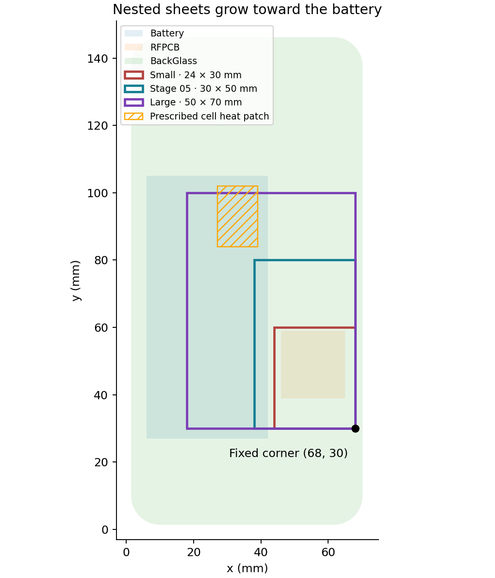
The sheet areas are 720, 1,500 and 3,500 mm². Their projected overlap with the battery is 0, 200 and 1,680 mm². Projected overlap means coupling across the modeled internal gap, not physical sheet-to-cell contact. The largest sheet reaches most of the prescribed cell heat patch at x = 27–39, y = 84–102 mm. Its upper edge ends at y = 100 mm.
Thickness and material properties stay fixed, so larger sheets necessarily add graphite mass, adhesive mass, thermal capacity and bonded area. They also redirect a larger share of internal gap paths from the back glass to the sheet. Those are physical consequences of this footprint change, not an isolated lateral-conductivity test; Stage 05 retains that separate control. Native FreeCAD and STEP checks confirm 67 valid, non-overlapping solids per size, 80 mm² of pad contact and bonded-sheet contact equal to each footprint area.
3 · Compare cover, cell average and cell peak together
| Case at 600 s | Area (mm²) | Cell overlap (mm²) | Cover max (°C) | Cell mean (°C) | Cell max (°C) | RF board max (°C) |
|---|---|---|---|---|---|---|
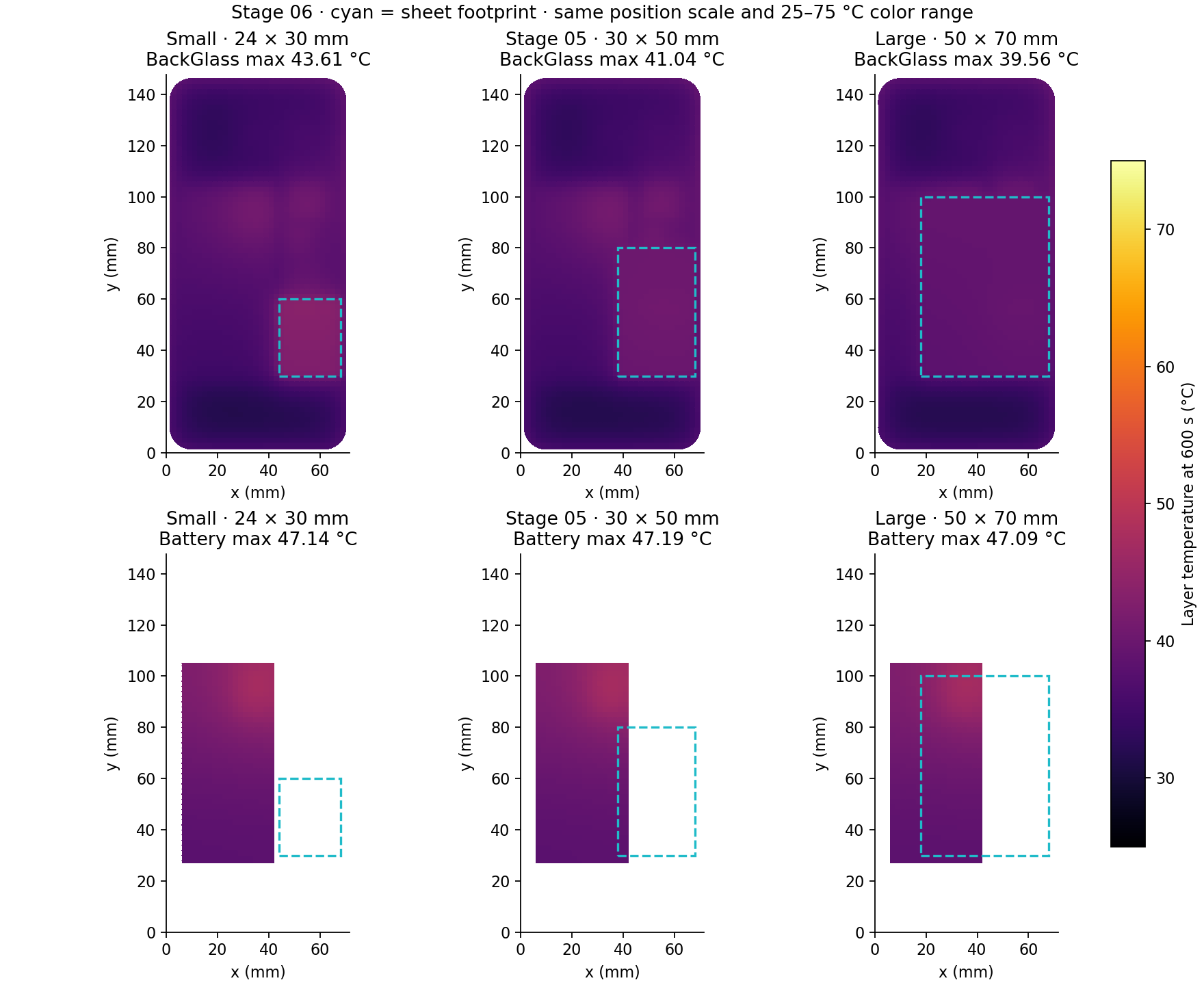
| Small · 24 × 30 mm | 720 | 0 | 43.61 | 40.95 | 47.14 | 57.01 |
| Stage 05 · 30 × 50 mm | 1500 | 200 | 41.04 | 41.02 | 47.19 | 55.02 |
| Large · 50 × 70 mm | 3500 | 1680 | 39.56 | 41.07 | 47.09 | 54.16 |
Relative to the 30 × 50 mm reference, the large sheet changes the cover maximum by -1.48 K, the cell average by +0.055 K, and the cell maximum by -0.109 K. A lower peak and a lower average are different objectives: redistribution can flatten a field without lowering every location.
4 · Follow the spreading and the changed heat paths
Gx = kxt Δy/Δx · Csheet = ρcpAt · Q̇ij = Gij(Ti − Tj)
The sheet conductance per square, kxyt = 0.08 W/K, is unchanged. More area supplies additional lateral paths and connects the RF-pad region to more of the cover and cell surroundings. The small sheet ends below the cell’s prescribed heat patch; the large sheet reaches that region. Local heat flow reverses where a hotter part faces a cooler sheet. The battery mean reflects the whole cell’s energy, while its maximum tracks its hottest control volume. Neither should be inferred from the other.
Why can the battery average rise while its peak falls? The independent cell-energy audit finds that the large sheet removes an additional 64.05 J through the graphite path and 16.13 J through the cell-to-midplate path over the first 600 s. But its larger footprint replaces direct cell-to-cover gap paths that had removed 81.82 J more in the reference. The combined change leaves 1.647 J more stored in the cell. Dividing by its unchanged 29.98944 J/K capacity gives the modeled +0.0549 K average rise. Locally, the sheet reaches the prescribed hot patch and lowers the peak, while other cell regions warm. The positive net cell-to-sheet flow at 600 s alone cannot explain the full temperature history.
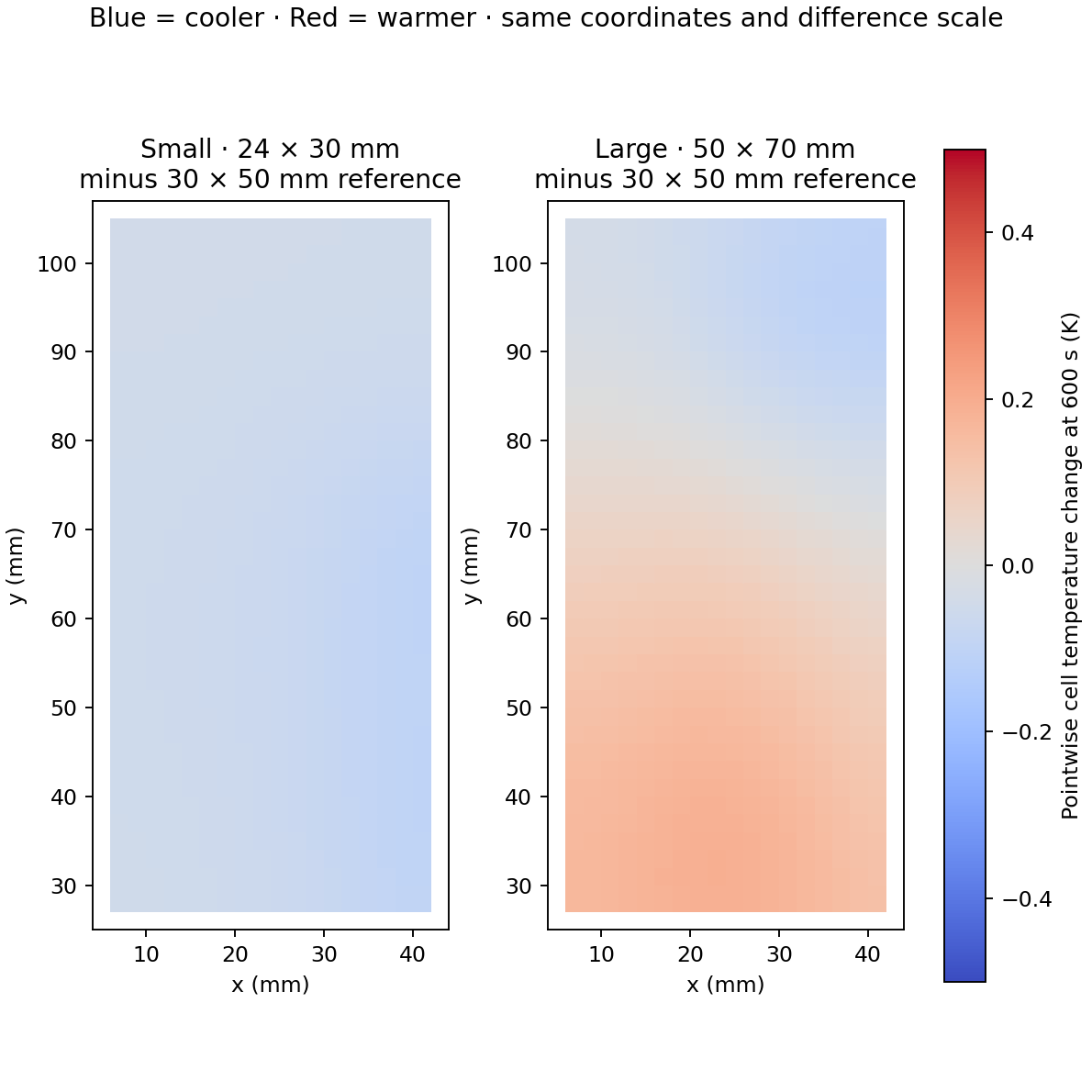
Difference maps compare the same cell control volumes at 600 s. The zero-centered scale is separate from the absolute-temperature maps. These are changes at fixed locations; the difference between component maxima in the table may compare different locations.
At 600 s the cover maximum occurs at the following control-volume centers: small (53.0, 57.0), reference (35.0, 95.0), large (70.1, 97.0) mm. These maxima may move between cases. They are layer temperatures, not resolved exterior skin or semiconductor junction temperatures.
| Case at 600 s | Cell → graphite (W) | Pad → graphite (W) | Adhesive → cover (W) | Stored energy (J) | Exterior loss (J) |
|---|---|---|---|---|---|
| Small · 24 × 30 mm | +0.00000 | 0.15672 | 0.22868 | 1409.63 | 840.37 |
| Stage 05 · 30 × 50 mm | -0.00194 | 0.17597 | 0.29142 | 1410.04 | 839.96 |
| Large · 50 × 70 mm | +0.15574 | 0.18214 | 0.52781 | 1413.12 | 836.88 |
Positive cell-to-graphite flow means the cell supplies net heat to the sheet; negative means the sheet supplies net heat to the cell. Zero in the small case denotes no projected cell-to-sheet path. Net values can hide simultaneous local flows in opposite directions. Adhesive-to-cover flow includes all sources coupled to the sheet, not just the RF pad. Each case receives exactly 2,250 J by 600 s; the stored-energy and exterior-loss columns sum to that input within numerical tolerance.
5 · Check the warm area, mass and the whole transient
| Case at 600 s | Cover >40 °C (mm²) | Cover >45 °C (mm²) | Cover mean (°C) | Graphite + adhesive mass (g) | Assembly modeled capacity (J/K) |
|---|---|---|---|---|---|
| Small · 24 × 30 mm | 1168 | 0 | 36.71 | 0.1512 | 96.6154 |
| Stage 05 · 30 × 50 mm | 1628 | 0 | 36.68 | 0.3150 | 96.7488 |
| Large · 50 × 70 mm | 0 | 0 | 36.64 | 0.7350 | 97.0908 |
A spreader redistributes energy and adds transient heat capacity. Its benefit depends on access to cooler regions and on the exterior heat-removal path. The 40 and 45 °C thresholds are map diagnostics, not safety or touch limits. Areas count whole finite-volume cells by their center temperatures; no interpolated contour boundary is implied.
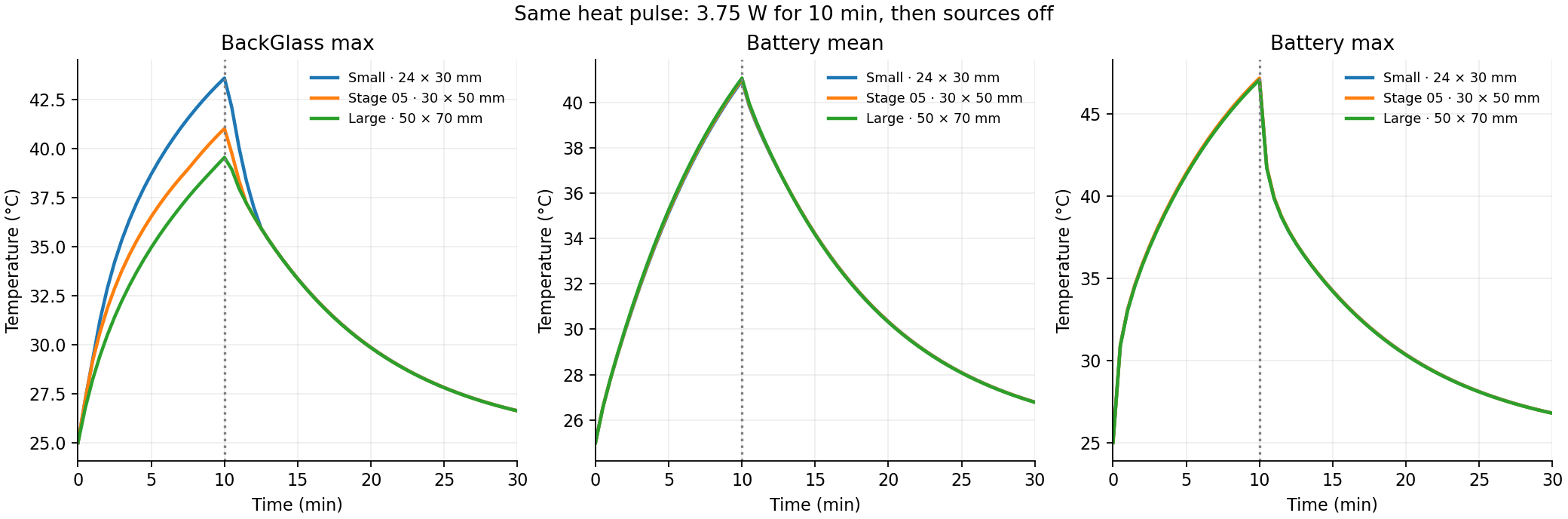
The table compares the same instant at the end of heating, not a steady state. Cooling continues after source shutoff and internal components can exchange stored heat. Use the timeline to inspect each saved time; full-precision component histories are available below.
6 · Test the numerical result before drawing a design conclusion
Every size is solved on a 2 mm grid with a 2 s backward-Euler step, then checked on a 1 mm grid and with a 1 s time step. Node counts are 10,070, 10,460 and 11,460; finer counts are 38,676, 40,236 and 44,236. The largest component-maximum grid difference at 600 s is 0.3447 K; the largest time-step difference is 0.00793 K. Maximum full-transient energy residual is 9.04e-10 J; isolated-source rises sum to the combined rise within 9.24e-14 K.
| Effect at 600 s | 2 mm change (K) | 1 mm change (K) | Effect sensitivity (K) |
|---|---|---|---|
| small − reference · BackGlass_max | +2.5759 | +2.3214 | 0.2545 |
| small − reference · Battery_mean | -0.0638 | -0.0621 | 0.0018 |
| small − reference · Battery_max | -0.0496 | -0.0476 | 0.0020 |
| large − reference · BackGlass_max | -1.4763 | -1.4121 | 0.0642 |
| large − reference · Battery_mean | +0.0549 | +0.0516 | 0.0033 |
| large − reference · Battery_max | -0.1086 | -0.1116 | 0.0030 |
These paired checks are especially important for small battery differences: compare the change itself across meshes rather than treating an unsigned mesh error as a hardware confidence interval. This stage identifies a useful footprint tradeoff in the assumed model; it does not establish an optimal product design or a battery safety margin.
Limits inherited from Stage 05: one temperature per layer control volume through thickness, lumped packages, constant properties, resistance-based internal air conduction and fixed linearized radiation, no resolved airflow, no nonlinear radiation, compression mechanics, electrochemistry or measured contact properties. Sheet and adhesive have finite heat capacity and no ambient sink. Experimental material/interface data and independent tests are still required for physical validation.
Reproduce and inspect the size comparison
Free Python, NumPy, SciPy, Shapely and Matplotlib solve the thermal network; FreeCAD provides CAD and ParaView reads the saved VTK. The archive includes the frozen Stage 05 reference, per-size meshes, conductance links, source maps, material assumptions and all fields. No commercial solver is required.
Read the README before running. The preserved Stage 05 spreader module supplies the stack implementation; run source/run_size_study.py for this stage.